Understanding Hierarchical Temporal Memory

Last year I did one project on Cognitive Healthcare which used Hierarchical Temporal Memory or HTM.Through this post, I have tried to put down my understanding of Numenta’s HTM. Before getting to it, it is important to understand the functioning of the neocortex to process sensory inputs from the physical world because HTM is inspired by the same.

HTM is inspired by neocortex

Human Neocortex

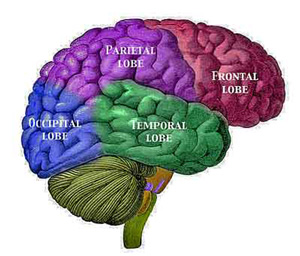
Broadly speaking, a brain is divided into four major lobes:

• the frontal lobe (associated with reward, attention, short-term memory tasks, planning, and motivation)
• the parietal lobe (involved in integrating sensory information from the various senses, and in the manipulation of objects in determining spatial sense and navigation)
• the occipital lobe (visual)
• the temporal lobe (involved with the senses of smell and sound, the processing of semantics in both speech and vision, including the processing of complex stimuli like faces and scenes, and plays a key role in the formation of long-term memory)

In humans, the neocortex is the size of a dinner napkin 2.5 mm thick and it is folded to fit inside our skull. Older parts of the brain that are below the neocortex are involved in the basic functions of life like eating, sleeping, and getting emotional. But that is not where intelligence resides.  The neocortex is the part that gives you memory and stores all the lessons that you learned.

Structure of neocortex

The neocortex is generally said to have six layers. Five of the layers contain cells and one layer is mostly connections. The image below (from Santiago Ramon y Cajal) shows a small slice of neocortex exposed using three different staining methods. The vertical axis spans the thickness of the neocortex, approximately 2mm. The left side of the image indicates the six layers. Layer 1, at the top, is the non-cellular level. The “WM” at the bottom indicates the beginning of the white matter, where axons from cells travel to other parts of the neocortex and other parts of the brain.

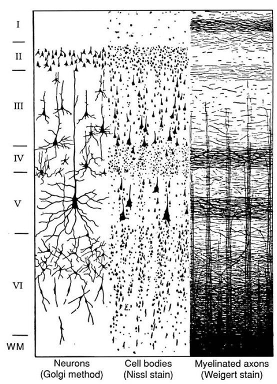
• Although Layer 2 and 3 look easily distinguished they are normally considered as one layer i.e, Layer 2/3.
• Layer 4 is the most well defined in those neocortical regions which are closest to the sensory organs.
• Layer 5 has the largest cells in the cortex.
• Layer 6 projects different sub-cortical areas and sends feedback to the thalamus.

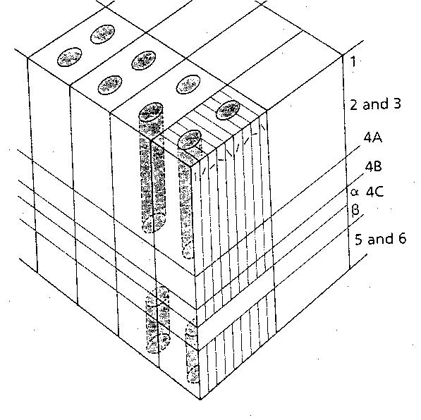
If you cut out any portion of neocortex and observe at cellular level, every portion looks alike no matter from where you cut it out from – visual, auditory, or any other part of brain – all the same. This tells us that the brain deals with the sensory inputs in an almost identical manner . It uses the same sets of algorithms for every kind of information. There is one more specialty about the structure of the neorocortex. It is observed that the neurons are aligned vertically in columns. And the neurons in the same column respond to the same type of input.

Mapping the Neocortex to the HTM Model

As there is a hierarchy of layers in neocortex, so is the case in HTM. The raw data is sensed by the lower levels and then the processed data is feed-forwarded to the next higher level in the hierarchy.

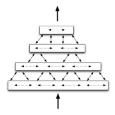
An HTM can be composed of just one region, or several regions with data being fed through them. The region itself is comprised of interconnected cells that can be in one of three states: *Active from feed-forward input. *Active from lateral input (a prediction) *Inactive.

The cells are stacked on top of each other in vertical columns forming a three dimensional grid:

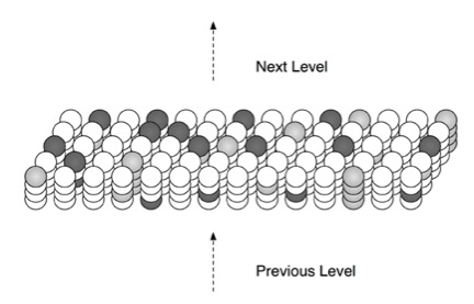
The HTM cortical learning algorithm shows that a layer of cells organized in columns can be a high-capacity memory of variable order state transitions. Stated more simply, a layer of cells can learn a lot of sequences. Columns of cells that share the same feed-forward response are the key mechanism for learning variable-order transitions.

Sparse Distributed Representations

The human cortex has about 20 – 30 billion neurons. At any point of time, the active neurons are just 2% of that number. Thus, information in the brain is always represented by a small percentage of active neurons within a large population of neurons. This kind of encoding is called a sparse distributed representation (SDR). HTM also uses SDRs. The input to an HTM region is always a distributed representation, but it may not be sparse, so the first thing an HTM region does is convert its input into a sparse distributed representation. We can represent an input as a SDR by an array of 1’s and 0’s . Each bit in the array represents a neuron or cell.

How are the predictions made?

The cells are grouped in vertical columns, and all the cells in a column get the same feed-forward input (either directly from the data, or the output from a lower HTM region). The input, as mentioned previously, is converted to a sparse distributed representation, and then each column gets a unique subset of that input (usually overlapping with other columns, but never the exact same subset). Cells also receive lateral input from other columns of cells. Which cells get activated within a column depends on a variety of factors, and the use of columns allows the HTM to create temporal contexts. This white paper explains:

By selecting different active cells in each active column, we can represent the exact same input differently in different contexts. A specific example might help. Say every column has 4 cells and the representation of every input consists of 100 active columns. If only one cell per column is active at a time, we have 4^100 ways of representing the exact same input. The same input will always result in the same 100 columns being active, but in different contexts different cells in those columns will be active.

Which cells in a column become active depends on the current activation state of those cells:

When a column becomes active, it looks at all the cells in the column. If one or more cells in the column are already in the predictive state, only those cells become active. If no cells in the column are in the predictive state, then all the cells become active. You can think of it this way, if an input pattern is expected then the system confirms that expectation by activating only the cells in the predictive state. If the input pattern is unexpected then the system activates all cells in the column as if to say “the input occurred unexpectedly so all possible interpretations are valid”.

Real neural networks contain inhibitory signals as well as excitatory ones. The same concept is applied in HTM regions as part of the lateral input that cells receive from their neighboring columns:

The columns with the strongest activation inhibit, or deactivate, the columns with weaker activation. (The inhibition occurs within a radius that can span from very local to the entire region.) The sparse representation of the input is encoded by which columns are active and which are inactive after inhibition. The inhibition function is defined to achieve a relatively constant percentage of columns to be active, even when the number of input bits that are active varies significantly.

Lateral input can inhibit as well as excite cells, and this is how HTM regions form predictions:

When input patterns change over time, different sets of columns and cells become active in sequence. When a cell becomes active, it forms connections to a subset of the cells nearby that were active immediately prior. These connections can be formed quickly or slowly depending on the learning rate required by the application. Later, all a cell needs to do is to look at these connections for coincident activity. If the connections become active, the cell can expect that it might become active shortly and enters a predictive state. Thus the feed-forward activation of a set of cells will lead to the predictive activation of other sets of cells that typically follow. Think of this as the moment when you recognize a song and start predicting the next notes.

The influence one cell has on another is moderated by the strength of the a virtual synapse between, which can have a decimal value between 0 and 1.

Tools to implement HTM : NuPIC

Numenta Platform for Intelligent Computing or NuPIC is an open source project based on HTM.It learns the time-based patterns in data , predicts future values and detects anomalies.You can very easily follow the instructions given on their website and start building your own application around NuPIC.

I hope you found this blog helpful.Cheers!