Target pose estimation and reaching using supervised learning
This is an ongoing project whose main goal is to teach manipulation tasks to the robot by observing humans perform the tasks. This observation is fed to the robot in the form of image sequences or a video. In this post I will try to explain some of the preliminary implementation of one part of the project that is estimating the target position.
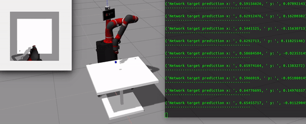
Fig 1. CNN predicts the target pose for reaching task
Environment
The simulation is set up in the Gazebo simulator. The robot being used is 7DOF Sawyer robot with an electronic gripper attached to the end-effector. A camera is placed on top of the workspace to capture images to be fed to the network. A table is also spawned in the world on top of which a blue cube randomly spawns.
Task
To predict the blue cube's position on the table and reach to that position.
Architecture
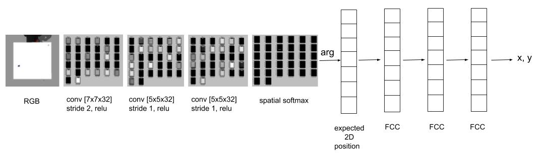
Fig 2. CNN architecture to predict cube position
The network consists of 3 convolutional layers which learn a bank of filters. These filters form a hierarchy of local image features. The convolution operation is followed by a rectifying nonlinearity of the form \(a_{cij}=\max(0, z_{ij})\) for each channel c and each pixel coordinate \((i,j)\). The third convolutional layer contains 32 response maps. These response maps are passed through a spatial softmax function of the form \(s_{cij} = {e^{a_{cij}}}/{\sum_{i^{'} j^{'}}{e^{a_{ci^{'}j^{'}}}}}\). Each output channel of the softmax is a probability distribution over the location of a feature in the image. To convert from this distribution to a coordinate representation \((f_{cx}, f_{cy} )\), the network calculates the expected image position of each feature, yielding a 2D coordinate for each channel: \(f_{cx} = \sum_{ij}{s_{cij}x_{ij}}\) and \(f_{cy} = \sum_{ij}{s_{cij}y_{ij}}\) where \((x_{ij}, y_{ij})\) is the image-space position of the point \((i, j)\) in the response map.
The spatial softmax and the expected position computation serve to convert pixel-wise representations in the convolutional layers to spatial coordinate representations, which can be manipulated by the fully connected layers into 3D positions.
Input image during test
For demonstration purpose, I randomly sampled two images from the test data set. As can be seen in the following figure, cube is spawned on two different positions on the table.
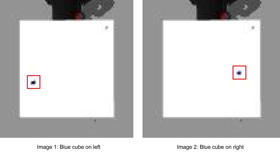
Fig 3. Input to the CNN
Spatial softmax for the two inputs looks as follows
- Image 1 (cube on left)
- Image 2 (cube on right)
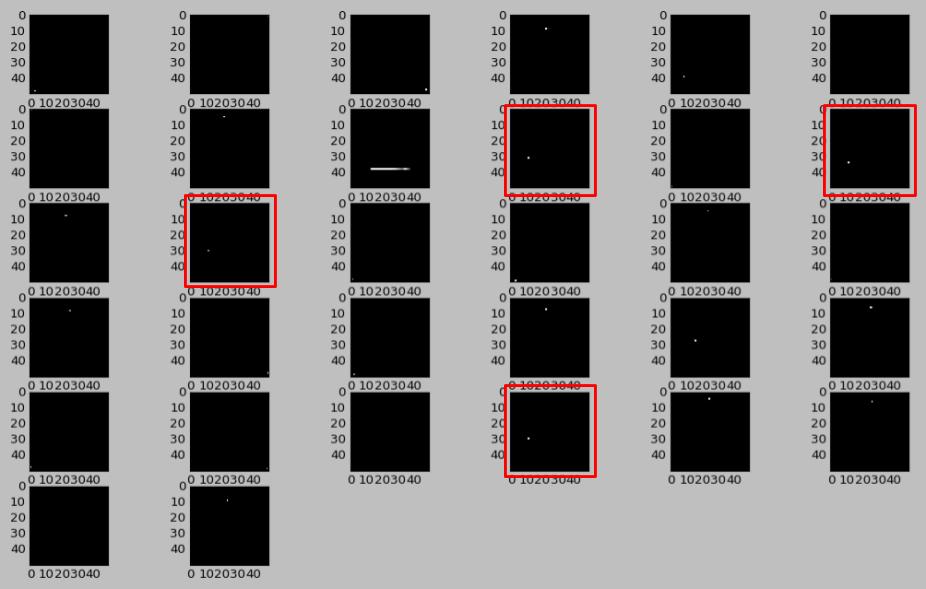
Fig 4. Spatial softmax for image 1
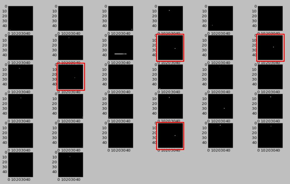
Fig 5. Spatial softmax for image 2
What you see in Fig 4. and Fig 5. are the results of softmax operation on the activation maps of third convolutional layers. This operation results in a probability distribution over features in each activation map. There are 32 activation maps in total because of the 32 filters used in the convolution operation. The softmax operation points to the area of maximum activation in each activation map i.e, the most important feature. The next step, as discussed before, is to calculate the expected 2D position of each feature.
Results
The results for image 1 are as follows:
predicted position : [ 0.72932047, -0.3483142 ]
true position : [0.72, -0.35]
test loss : 4.485624e-05
As can be seen from the results, the network predicts the cube's position pretty well. This acts as the target position for the robot's end effector. The IK solver calculates the joint angles to be reached and the robot's controller tries to reach this configuration.
Reference
Levine, Sergey, Chelsea Finn, Trevor Darrell, and Pieter Abbeel. "End-to-end training of deep visuomotor policies." The Journal of Machine Learning Research 17, no. 1 (2016): 1334-1373.